How ECUs calculate fuel delivery

Calibrating an engine is usually predictable, until something changes. Swap injectors, change fuels, or add flex-fuel support, and the engine that was dialled in last week can run poorly, even though your injector and fuel data looks correct. The reason comes back to how the ECU calculates fuel delivery and where errors in that calculation end up stored.

First, you swap injectors. The old ones were running fine. You fit larger units, enter the new flow rate from the manufacturer's spec sheet, and the engine runs inconsistently across the map. The new injector data looks correct. Something's still off.

Second, you change fuels. The engine was dialled in on pump gas, you switch to E85, you adjust the stoichiometric AFR and density and expect a straightforward retune. The mixture targets are achievable, but the VE table shape feels different at specific load points. The table you had before doesn't transfer cleanly even after accounting for the stoich change.

Both scenarios come back to how the ECU calculates fuel delivery and where errors in that calculation end up stored. Understanding this changes how you approach calibration, what you verify before touching the VE table, and why hardware or fuel changes sometimes force much bigger retunes than they should.

In this article

• Two ECU architectures
• The airflow model
• The fuel model
• Injector characterisation
• How fuel model errors propagate
• Practical takeaways
• Key points

Two ECU architectures

There are two primary ECU architectures across the majority of ECUs. These are Millisecond based or Airflow based.

Millisecond-based ECUs use a main fuel table that outputs injector pulse width directly. This table is a fuel model table, not an airflow model table. There's no separate airflow calculation. Volumetric efficiency, injector flow, fuel stoichiometry, heat of vaporisation (HoV), and target lambda all collapse into one tuned table that the calibrator shapes until the wideband reads correctly. Some platforms label this table "VE" even though it isn't a VE table in the airflow-estimation sense. It's a pulse-width table with everything baked in. These systems work, but nothing downstream can change without retuning the whole thing.

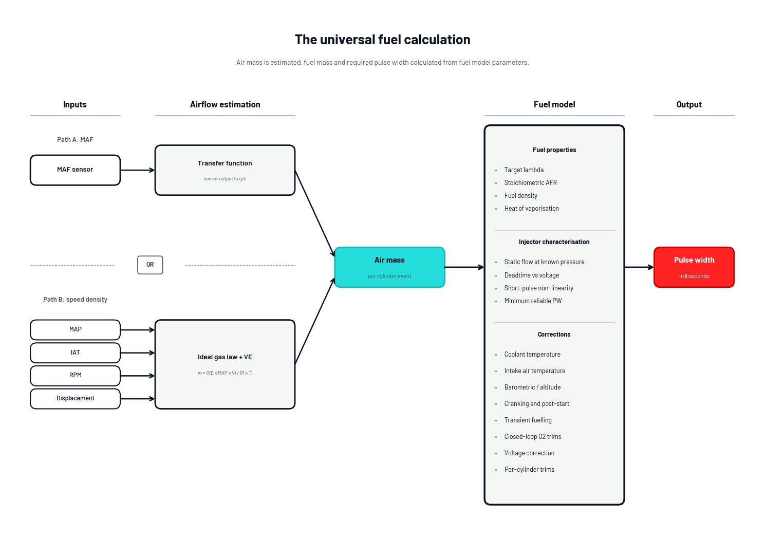
Airflow-based ECUs split the calculation into two stages. First the ECU estimates the air mass entering the cylinder. Then a separate fuel model determines the required fuel mass to achieve the target lambda, applies any appropriate corrections, and then calculates the required injector pulse width. The rest of this article covers airflow-based ECUs, because that's where most modern standalone and OEM systems live, and it's where the two-layer structure creates both the leverage and the failure modes.

One modern variant exists. Torque-based ECUs wrap the airflow model inside a torque request system. The driver's pedal input becomes a torque request, the ECU calculates the air mass needed to produce that torque, and the fuel model still converts air to fuel below that. The fuel model layer works the same way regardless of what sits above the airflow estimate.

The airflow model

Two primary methods exist for estimating air mass. These are Mass Airflow sensor and Speed Density.

Mass airflow sensing uses a sensor in the intake tract to measure airflow directly, typically via a heated element whose cooling rate correlates to mass flow. The sensor output maps to grams per second through a calibration curve called the transfer function. Air mass per cylinder event is derived from that overall flow rate, engine speed, and the number of cylinders.

In a Speed Density system there is no direct air mass measurement. Instead, the ECU calculates air mass from the ideal gas law using manifold absolute pressure, intake air temperature, engine displacement, and a volumetric efficiency (VE) term. The VE here is a calibrated correction factor, stored in the VE Table, representing the ratio of actual air inducted to the theoretical possible for that engine. It's the tunable term that aims to match the calculation to reality.

The practical difference is that MAF measures and speed density calculates. MAF accuracy holds when the sensor and intake geometry stay consistent but degrades when either changes. Aftermarket intakes, boost past a MAF sensor, or fuelling past the sensor all compromise the measurement. Speed density doesn't care about intake geometry but depends entirely on having the VE table right across the full operating range. Which approach an ECU uses affects where errors can hide. The fuel model sits after airflow estimation regardless of which method produced it.

The fuel model

The fuel model is a separate layer from the VE table. Treating them as the same thing is where most calibration problems start.

Once airflow has been calculated or estimated, the fuel model is used to determine the injector pulse width required to achieve or maintain the target lambda. It contains several parameters, and all of them must be set correctly for the calculation to be accurate.

Target lambda is the mixture the ECU aims for, varied by operating region (cruise, WOT, warmup, decel, overrun).

Stoichiometric AFR is fuel-dependent. Around 14.7 for gasoline, 9.76 for E85, and 6.47 for methanol. If the ECU doesn't know what fuel it's running, then calculating the required fuel mass will be wrong by the ratio of the assumed to actual stoichiometric value. Think straight gasoline vs E10 which will have a fuel mass difference of around 4 percent.

Fuel density is also fuel-dependent. It converts fuel mass to fuel volume, which matters because injectors are rated in volume flow.

Heat of vaporisation describes how much energy fuel absorbs as it evaporates in the intake port or cylinder. That evaporation cools the charge, raises density, and increases the air mass the engine actually inducts compared to what would happen with a non-evaporating fuel. Gasoline's HoV is around 350 kJ/kg. E85's is around 840 kJ/kg. The effect is larger with E85, because each kilogram of E85 cools more, and because more kilograms are burned per gram of air. Some ECUs model this explicitly. Many don't.

Injector flow rate at a specified differential pressure is where proper injector characterisation starts, and where most fuel model errors originate.

Several correction layers sit on top of these core parameters. Coolant temperature compensation enriches the mixture during warmup and leans it out as the engine reaches operating temperature. Intake air temperature compensation adjusts fuel quantity as charge density changes with air temperature. Barometric compensation handles changes in ambient air density with altitude. Cranking and post-start enrichment provide the extra fuel needed to light off a cold engine. Transient fuelling handles the acceleration enrichment required during rapid throttle tip-in and the fuel cut during deceleration. Closed-loop O2 trims apply ongoing correction when narrowband or wideband feedback is active. Voltage correction and per-cylinder trims sit at the bottom of this stack. Every one of these corrections is a tunable layer in the fuel model, and every one can carry error if not set correctly.

Injector characterisation

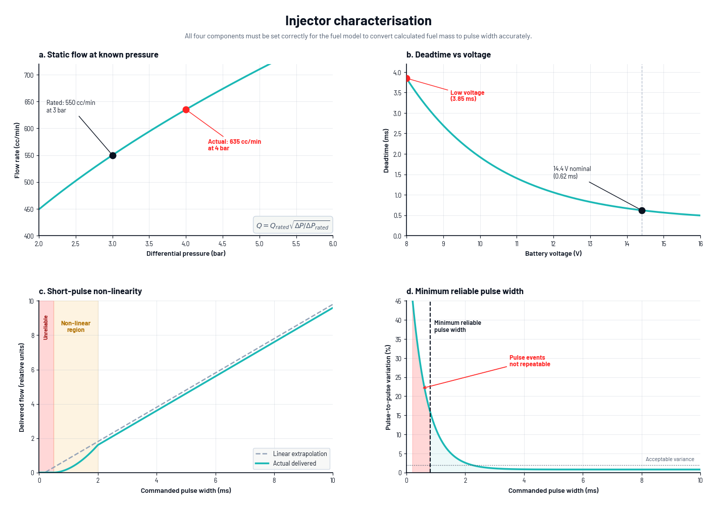
Proper injector characterisation has four components. All four matter and missing any of them guarantees error in the fuel model.

Static flow rate at a specified differential pressure is the starting point. The typical reference is 3 bar (43.5 psi). Some aftermarket data is rated at 4 bar. Actual flow through the injector scales with the square root of the pressure ratio across the injector, which just means that to double the flow you need 4 times the pressure. A 550 cc/min injector rated at 3 bar, for example, delivers about 635 cc/min at 4 bar base pressure. The injector itself hasn't changed. The rated flow has, because the test condition is different.

Flow data without a reference pressure is meaningless. An injector rated at 3 bar and the same physical injector rated at 4 bar are functionally different numbers in a fuel model.

Deadtime as a function of voltage is the second component. Deadtime is the delay between the ECU signal and the injector beginning to flow fuel. Lower battery voltage means slower opening times and a longer deadtime value. The deadtime table typically spans roughly 8V to 16V and having the wrong deadtime values will shift every calculated pulse width by a fixed amount. This matters more at short pulse widths (idle and light loads) where that fixed amount is a larger percentage of the total event.

Short-pulse non-linearity is the third. Below roughly 1.5 to 2 ms pulse width, injectors don't flow linearly because the opening and closing transitions dominate the event rather than the fully-open flow rate. Good characterisation includes a non-linearity curve or short-pulse correction table for this region. Idle and light cruise often operate here and, again, are the most affected by this non-linear behaviour.

Minimum reliable pulse width is the fourth. Below a certain point, pulse widths become unrepeatable and the ECU can't accurately deliver the requested fuel mass. Idle, decel, and overrun regions often operate near this limit on larger injectors. Characterisation identifies where that limit is.

With all four set correctly, the fuel model takes calculated air mass, applies target lambda and fuel properties to get fuel mass, then applies the injector characterisation to get pulse width. When any part is wrong, something else has to absorb the error. That something is usually the VE table.

How fuel model errors propagate

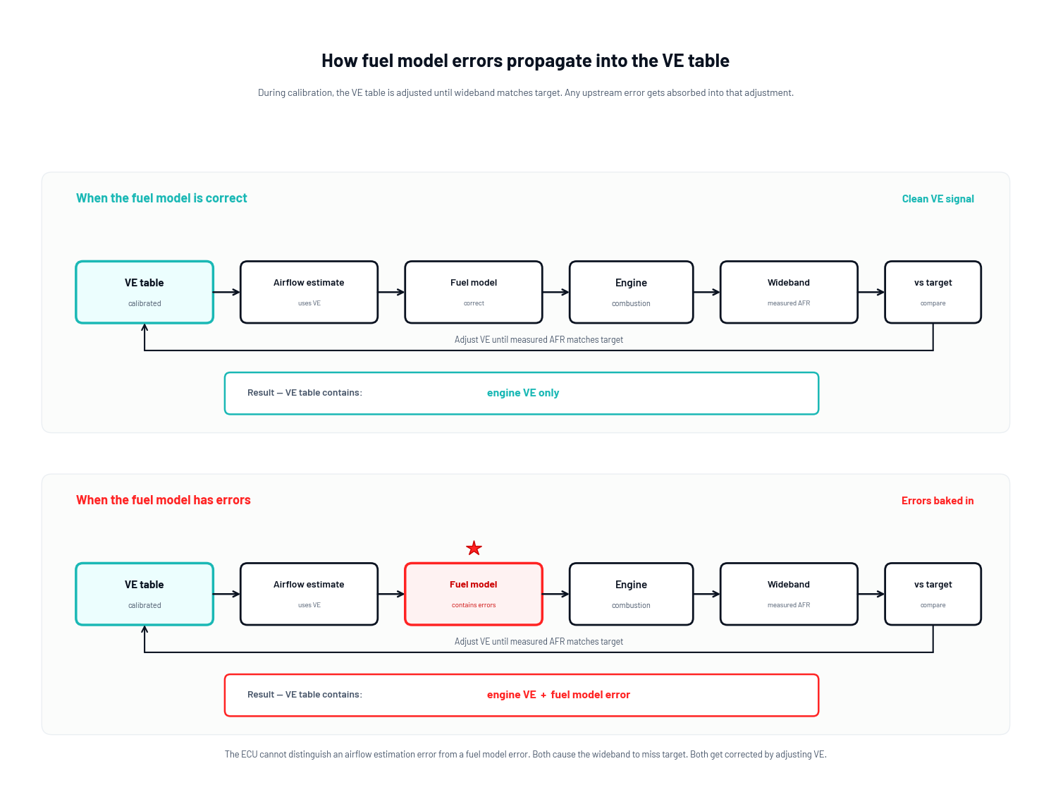
The VE table is where calibration work ends up reflecting real engine behaviour. When you tune VE, you're adjusting the airflow estimate until calculated fuel matches target lambda at the wideband. If the airflow estimate is genuinely off by 5%, for example, VE is adjusted and fuelling is corrected. That's what the VE table is for.

The problem is, if the fuel model is off by 5%, it's the VE table that also ends up compensating for it. The ECU can't tell the difference between an incorrect airflow estimate and a fuel model that's off. Both cause the mixture at the wideband to deviate from target, and both get corrected by adjusting VE. Errors in the fuel model show up as errors in the VE table, and once they're there, they can't be separated from real VE data.

New injectors have a different static flow rate, different deadtime curves, and different short-pulse width behaviour. If any of the old injector data was absorbed into the VE table, the new setup won't work the way that you expect. The VE table that was accurate for the old injector becomes unusable for the new one, and a full retune is needed. Not ideal.

Changing fuels can also force a full VE retune outside of flex-fuel setups. Switching from pump gas to E85 changes stoichiometric AFR, density, and HoV. If the fuel model includes stoichiometric AFR and density but not HoV, the VE table absorbs the charge-cooling effect. When you switch fuels, the table is calibrated for the old fuel's HoV and is wrong for the new one.

The VE table stops being a model of the engine and starts being a collection of compensations for everything else. You can't reason about it anymore.

Flex-fuel systems handle the HoV case differently. With an ethanol content sensor and 4D VE tables indexed by ethanol percentage, each layer of the VE structure gets calibrated at the ethanol level it corresponds to. If the fuel model doesn't include HoV, the HoV effect at each ethanol level is baked into that layer's VE table during initial calibration. The system works because the table itself is referencing the variable that's changing, and a different layer takes over when the ethanol content changes. Outside a flex-fuel setup only one VE table exists, so switching fuels can force a retune depending on the fuels and how far out it is.

VE tables don't transfer between similar engines for the same reason. A clean VE table from a built engine should be portable to a similar build. In practice it often isn't, and the reason usually isn't the engine. It's that one setup had different injector data, different fuel parameters, or different deadtime than the other, and those differences are now baked into the VE table.

Diagnostic signal also suffers. When something goes wrong on a tune whose VE carries fuel model errors, the data is harder to read. A lean spot at a specific load point could be a VE issue, a sensor drift, a fuel delivery problem, or a fuel model error that's now out of range. You can't tell which without unwinding the calibration, and that usually isn't practical.

Neither architecture is immune. In a MAF system, fuel model errors show up in the fuel trims and correction tables. In a speed density system, they end up in the VE table directly, which makes them easier to see but also harder to unwind. Whichever system you have, the fuel model needs to be right before you start tuning.

Practical takeaways

Set the fuel model before you tune the VE table, not after.

Before calibration starts, verify the injector specification at a known differential pressure. Cross-reference flow data against multiple sources where possible. Manufacturer data at a stated reference pressure is the starting point, not a number typed from memory or copied from a forum post.

Verify deadtime data across the voltage range. Default or guessed deadtime tables are one of the most common sources of error in the fuel model. Good injector datasets include measured deadtime at multiple voltages.

If the ECU supports short-pulse non-linearity correction and the application runs large injectors, use it. Skipping it forces the VE table to carry idle-region distortion that doesn't belong there.

Check HoV handling. If the ECU models HoV and the application uses a fuel with significant deviation from gasoline, enable it. If the ECU doesn't model HoV, just be aware that the VE table will carry that information, and that changing fuels may require a retune.

Set target lambda, stoichiometric AFR, and fuel density correctly before touching VE. Changing any of these mid-calibration reshuffles every subsequent VE adjustment.

Telling a fuel model error from a real VE error comes down to the pattern. A fuel model error shows up as a consistent bias across a broad region of the table. A real VE error is usually localised, reflecting something specific about the engine like cam overlap or intake resonance. If you see a large area of the table that's all off in the same direction by a similar amount, the fuel model is the first place to look. If you see a distinct feature in one region, the engine is telling you something.

Key points

• Ms-based ECUs use a single fuel model table that outputs pulse width directly. It's a fuel model table, not an airflow model table, and everything gets baked in.
• Airflow-based ECUs split the calculation. Air mass first, then fuel mass via a separate fuel model, then pulse width.
• The fuel model contains fuel properties (target lambda, stoich, density, HoV), injector characterisation, and multiple correction layers (coolant, IAT, baro, cranking, transient, closed-loop trims, voltage, per-cylinder). It's a distinct layer from the VE table.
• Proper injector characterisation means static flow at a specified pressure, deadtime vs voltage, short-pulse non-linearity, and minimum reliable pulse width. All four matter.
• Errors in the fuel model propagate into the VE table during calibration. The ECU can't tell a fuel delivery error from an airflow estimate error, so both get corrected the same way.
• Injector swaps and fuel changes force full VE retunes when the fuel model was carrying errors. Flex-fuel setups with 4D VE tables indexed by ethanol content handle fuel HoV changes structurally. Single-fuel setups don't.
• Set the fuel model before the VE table, not after.